Blog post for Week 4 of Machine Learning for Data Analysis (Coursera)
What is K-Means Cluster analysis?
The goal of cluster analysis is to group or cluster observations into subsets based on the similarity of responses on multiple variables such that each observation belongs to a group in which it shares the most similarity in mean with its members (less in-class variance) and is most dissimilar between other groups (more variance between clusters). This is a unsupervised machine learning method as the label (response) is unknown. A measure of cluster similarity is defined by how close the observations are to each other by the Euclidean distance which draws a straight line from observation to observation.

k-means clustering is iterative rather than hierarchical, clustering algorithm which means at each stage of the algorithm data points will be assigned to a fixed number of clusters (contrasted with hierarchical clustering where the number of clusters ranges from the number of data points (each is a cluster) down to a single cluster for types Agglomerative and Divisive).
Real world examples of k-means clustering: finding certain segments of customers for targeted advertisements to offer tailored incentives in marketing analytics.
Limitations of k-means clustering: need to specify the number of clusters upfront by subjective guessing, results can changed depending on the location of the initial centroids and this analysis method is not recommended if there are a lot of categorical variables. K-means assumes that clusters are spherical, distinct and approximately equal in size.
Alternatives to k-means:
- DBSCAN for non-spherical shapes, and uneven sizes
- Agglomerative clustering for many clusters, non-eucledian distances
- Additional methods
Analysis process
-
Dataset selection: The poker hand dataset from UCI Machine Learning was selected for this analysis which aims to predict poker hands. Each record is an example of a hand consisting of five playing cards drawn from a standard deck of 52. Each card is described using two attributes (suit and rank), for a total of 10 predictive attributes. There is one Class attribute that describes the “Poker Hand”. The order of cards is important, which is why there are 480 possible Royal Flush hands as compared to 4 (one for each suit - explained in Web Link).
-
Data Management: There are 1025010 instances, 10 attributes, 1 class variable and No missing values. The “Sx” columns indicate the suit of a Card (Heart, Spades, Diamonds, Clubs). The “Cx” columns indicate the numerical rank (1-13) representing (Ace, 2, 3, …, Queen, King). The data was read into python with the
urlliband therequest.urlretrievefunction to save the train and test (already partitioned by the researchers) to a local file and read in the file as apandasdataFrame. -
Subset & standardize clustering variables: The cluster variables were sub-setted from the class variable and standardized so that the Suit and Rank would each have equal contribution regardless of scale.
-
Split into test and training: The data has already been partitioned into a train and test data sets. 25010 observations for training, 1,000,000 for testing.
-
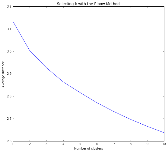
Calculate k-means for 10 clusters, due to the 10 possible class outcomes for poker hands (to see which is the optimal amount to use eventually as parameter tuning) then plot average distance from observations from the cluster centroid to use the Elbow Method to identify number of clusters to choose.
-
Interpretation of the selected 2 cluster solution indicating that a comparable reduction in average distance from the centroid of each cluster appears in 2 clusters as opposed to 10 clusters leading to a parsimonious model. So despite there being 10 types of poker hand there seems to be 2 clusters that the observations align to.
-
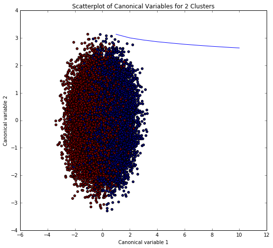
Visualize the clusters in a scatter plot to view potential overlapping (poor between-class variance) in terms of their location in the p dimensional space through graphing the 10 dimensions of the but since we can not effectively show all of them in a scatter plot we will use canonical discriminate analysis which is a data reduction technique that creates a smaller number of variables that are linear combinations of the 10 clustering variables (latent) that summarize between-class variation similar to principal component analysis summarize total variation and canonical correlation which describes the relationship between two sets of variables. The canonical variables are ordered in terms of proportion of variance and the clustering variable that is accounted for by each of the canonical variables. The first canonical variable will account for the largest proportion of variance - and so on for the second canonical variable representing the 2nd largest.
-
Merge cluster assignment with clustering variables to examine cluster variable means by cluster to see if they are distinct and meaningful.
-
Calculate clustering variables (Suit and Rank) means by cluster. From viewing the means for each variable you can examine and compare each cluster and how its members are similar to the group.
-
Validate clusters in training data by examining cluster differences in CLASS using ANOVA and Diagnostic tests: Tukey test of significance (find means that are significantly different from each other), Durbin-Watson (used to detect the presence of autocorrelation), R-squard (proportion of the variance).
Results
The k-means analysis was performed to identify underlying subgroups of poker hands (e.g. winning hands versus losing hands) based on 10 attributes which describe the the card suit (e.g. Diamonds) and the numerical rank (e.g. Ace). the elbow graph below was a key step in evaluating which amount for clusters were appropriate or at which point-bend would the optimal reduction in average distance of the variable observations were from a centroid. Several evaluations of the which amount of clusters were tested through parameter tuning to refine the model. The canonical variables plot shows overlapping clusters yet tight within group relationship.
This was a difficult classification dataset as indicated from the original researchers as the probability and over-sampling of some hands in the train set due to the low exposure (e.g. 4 royal flush hands). Poker is a probabilistic game of chance, skill and luck all play important factors in “winning-ness”. It’s difficult to detect underlying clusters with this analysis & dataset because of the unique possible hands and the lack of rank between the hands.
Here are the probabilities of getting a certain hand:
| Poker Hand | # of hands | Probability | # of combinations |
|---|---|---|---|
| Royal Flush | 4 | 0.00000154 | 480 |
| Straight Flush | 36 | 0.00001385 | 4320 |
| Four of a kind | 624 | 0.0002401 | 74880 |
| Full house | 3744 | 0.00144058 | 449280 |
| Flush | 5108 | 0.0019654 | 612960 |
| Straight | 10200 | 0.00392464 | 1224000 |
| Three of a kind | 54912 | 0.02112845 | 6589440 |
| Two pairs | 123552 | 0.04753902 | 14826240 |
| One pair | 1098240 | 0.42256903 | 131788800 |
| Nothing | 1302540 | 0.50117739 | 156304800 |
| Total | 2598960 | 1.0 | 311875200 |
Additional Documents
- Jupyter Notebook
- Python script
- Excel csv files: train, test
Python code
# load libraries
from pandas import Series, DataFrame
import pandas as pd
import numpy as np
import matplotlib.pylab as plt
from sklearn.cross_validation import train_test_split
from sklearn import preprocessing
from sklearn.cluster import KMeans
import urllib.request
from pylab import rcParams
rcParams['figure.figsize'] = 9, 8

'''
GET DATA
'''

# read training and test data from the url link and save the file to your working directory
url = "http://archive.ics.uci.edu/ml/machine-learning-databases/poker/poker-hand-training-true.data"

urllib.request.urlretrieve(url, "poker_train.csv")

url2 = "http://archive.ics.uci.edu/ml/machine-learning-databases/poker/poker-hand-testing.data"

urllib.request.urlretrieve(url2, "poker_test.csv")

# read the data in and add column names
data_train = pd.read_csv("poker_train.csv", header=None,
                        names=['S1', 'C1', 'S2', 'C2', 'S3', 'C3','S4', 'C4', 'S5', 'C5', 'CLASS'])

data_test = pd.read_csv("poker_test.csv", header=None,
                        names=['S1', 'C1', 'S2', 'C2', 'S3', 'C3','S4', 'C4', 'S5', 'C5', 'CLASS'])

'''
EXPLORE THE DATA
'''
# summary statistics including counts, mean, stdev, quartiles for the training dataset
data_train.head(n=5)
data_train.dtypes # data types of each variable
data_train.describe()

'''
SUBSET THE DATA
'''
# subset clustering variables
cluster=data_train[['S1', 'C1', 'S2', 'C2', 'S3', 'C3','S4', 'C4', 'S5', 'C5']]

'''
STANDARDIZE THE DATA
'''
# standardize clustering variables to have mean=0 and sd=1 so that card suit and
# rank are on the same scale as to have the variables equally contribute to the analysis
clustervar=cluster.copy() # create a copy
clustervar['S1']=preprocessing.scale(clustervar['S1'].astype('float64'))
clustervar['C1']=preprocessing.scale(clustervar['C1'].astype('float64'))
clustervar['S2']=preprocessing.scale(clustervar['S2'].astype('float64'))
clustervar['C2']=preprocessing.scale(clustervar['C2'].astype('float64'))
clustervar['S3']=preprocessing.scale(clustervar['S3'].astype('float64'))
clustervar['C3']=preprocessing.scale(clustervar['C3'].astype('float64'))
clustervar['S4']=preprocessing.scale(clustervar['S4'].astype('float64'))
clustervar['C4']=preprocessing.scale(clustervar['C4'].astype('float64'))
clustervar['S5']=preprocessing.scale(clustervar['S5'].astype('float64'))
clustervar['C5']=preprocessing.scale(clustervar['C5'].astype('float64'))

# The data has been already split data into train and test sets
clus_train = clustervar
'''
K-MEANS ANALYSIS - INITIAL CLUSTER SET
'''
# k-means cluster analysis for 1-10 clusters due to the 10 possible class outcomes for poker hands
from scipy.spatial.distance import cdist
clusters=range(1,11)
meandist=[]

# loop through each cluster and fit the model to the train set
# generate the predicted cluster assingment and append the mean distance my taking the sum divided by the shape
for k in clusters:
    model=KMeans(n_clusters=k)
    model.fit(clus_train)
    clusassign=model.predict(clus_train)
    meandist.append(sum(np.min(cdist(clus_train, model.cluster_centers_, 'euclidean'), axis=1))
    / clus_train.shape[0])

"""
Plot average distance from observations from the cluster centroid
to use the Elbow Method to identify number of clusters to choose
"""
plt.plot(clusters, meandist)
plt.xlabel('Number of clusters')
plt.ylabel('Average distance')
plt.title('Selecting k with the Elbow Method') # pick the fewest number of clusters that reduces the average distance

# Interpret 2 cluster solution
model3=KMeans(n_clusters=2)
model3.fit(clus_train) # has cluster assingments based on using 3 clusters
clusassign=model3.predict(clus_train)

# plot clusters
''' Canonical Discriminant Analysis for variable reduction:
1. creates a smaller number of variables
2. linear combination of clustering variables
3. Canonical variables are ordered by proportion of variance accounted for
4. most of the variance will be accounted for in the first few canonical variables
'''
from sklearn.decomposition import PCA # CA from PCA function
pca_2 = PCA(2) # return 2 first canonical variables
plot_columns = pca_2.fit_transform(clus_train) # fit CA to the train dataset
plt.scatter(x=plot_columns[:,0], y=plot_columns[:,1], c=model3.labels_,) # plot 1st canonical variable on x axis, 2nd on y-axis
plt.xlabel('Canonical variable 1')
plt.ylabel('Canonical variable 2')
plt.title('Scatterplot of Canonical Variables for 2 Clusters')
plt.show() # close or overlapping clusters idicate correlated variables with low in-class variance but not good separation. 2 cluster might be better.

"""
BEGIN multiple steps to merge cluster assignment with clustering variables to examine
cluster variable means by cluster
"""
# create a unique identifier variable from the index for the
# cluster training data to merge with the cluster assignment variable
clus_train.reset_index(level=0, inplace=True)
# create a list that has the new index variable
cluslist=list(clus_train['index'])
# create a list of cluster assignments
labels=list(model3.labels_)
# combine index variable list with cluster assignment list into a dictionary
newlist=dict(zip(cluslist, labels))
newlist
# convert newlist dictionary to a dataframe
newclus=DataFrame.from_dict(newlist, orient='index')
newclus
# rename the cluster assignment column
newclus.columns = ['cluster']

# now do the same for the cluster assignment variable create a unique identifier variable from the index for the
# cluster assignment dataframe to merge with cluster training data
newclus.reset_index(level=0, inplace=True)
# merge the cluster assignment dataframe with the cluster training variable dataframe
# by the index variable
merged_train=pd.merge(clus_train, newclus, on='index')
merged_train.head(n=100)
# cluster frequencies
merged_train.cluster.value_counts()

"""
END multiple steps to merge cluster assignment with clustering variables to examine
cluster variable means by cluster
"""

# FINALLY calculate clustering variable means by cluster
clustergrp = merged_train.groupby('cluster').mean()
print ("Clustering variable means by cluster")
print(clustergrp)

'''
validate clusters in training data by examining cluster differences in CLASS using ANOVA
first have to merge CLASS of poker hand with clustering variables and cluster assignment data
'''
# split into test / train for class
pokerhand_train=data_train['CLASS']
pokerhand_test=data_test['CLASS']
# put into a pandas dataFrame
pokerhand_train=pd.DataFrame(pokerhand_train)
pokerhand_test=pd.DataFrame(pokerhand_test)
pokerhand_train.reset_index(level=0, inplace=True) # reset index
merged_train_all=pd.merge(pokerhand_train, merged_train, on='index') # merge the pokerhand train with merged clusters
sub1 = merged_train_all[['CLASS', 'cluster']].dropna()

import statsmodels.formula.api as smf
import statsmodels.stats.multicomp as multi

# respone formula
pokermod = smf.ols(formula='CLASS ~ C(cluster)', data=sub1).fit()
print (pokermod.summary())

print ('means for Poker hands by cluster')
m1= sub1.groupby('cluster').mean()
print (m1)

print ('standard deviations for Poker hands by cluster')
m2= sub1.groupby('cluster').std()
print (m2)

mc1 = multi.MultiComparison(sub1['CLASS'], sub1['cluster'])
res1 = mc1.tukeyhsd()
print(res1.summary())