Blog post for Week 2 of Machine Learning for Data Analysis (Coursera)
What is Random Forest?
Random forests are predictive models that allow for a data driven exploration of many explanatory variables in predicting a response or target variable. Random forests provide importance scores for each explanatory variable and also allow you to evaluate any increases in correct classification with the growing of smaller and larger number of trees.
Analysis Process
The ‘Adult’ dataset from the UCI Machine Learning Repository which predicts whether income exceeds $50K/yr based on census data was chosen for this exercise. The dataset includes 14 variables (categorical and continuous) and 48842 observations.
The data was downloaded from http://archive.ics.uci.edu/ml/machine-learning-databases/adult/adult.data via excel (Data > Get External Data > From web). The column names were added and the missing values previously encoded as ‘?’ were replaced with a blank space and saved as a csv file.
The csv file was read into R using the readr package and the target (y) response of <=50k or >50k was made into a binary 0, 1 response. The remaining eligible factors (categorical) were transformed into a design matrix (exploded out into 0’s, 1’s) with the model.matrix() function.
R Code:
# data has been modified in excel initially to remove NA's as ? to '' and colnames have been added
library(readr)
adult <- read_csv("C:/Users/JD87417/Desktop/python work/Coursera/adult_income.csv")
View(adult)
adult$income_target_binary <- ifelse(adult$income_target == ">50K", 1, 0)
adult2 <- model.matrix(income_target_binary ~., data = adult)
adult2 <- as.data.frame(adult2)
dput(colnames(adult2)) # get colnames print out for python format
colnames(adult2)[98] = "income_target_50k"
write_csv(x=adult2, path="C:/Users/JD87417/Desktop/python work/Coursera/adult2_income.csv")
The python methodology utilized pandas, numpy, sklearn to build the Random Forest.
Results
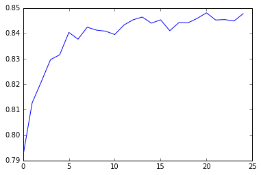
The explanatory variables with the highest relative importance scores were fnlwgt, age, capital_gain, education_num, raceWhite. The accuracy of the random forest was 85%, with the subsequent growing of multiple trees rather than a single tree, adding little to the overall accuracy of the model, and suggesting that interpretation of a single decision tree may be appropriate.
Additional Documents
Python code
# import libraries: dataframe manipulation, machine learning, os tools
from pandas import Series, DataFrame
import pandas as pd
import numpy as np
import os
import matplotlib.pylab as plt
from sklearn.cross_validation import train_test_split
from sklearn.tree import DecisionTreeClassifier
from sklearn.metrics import classification_report
import sklearn.metrics
 # Feature Importance
from sklearn import datasets
from sklearn.ensemble import ExtraTreesClassifier

# change working directory to where the dataset is
os.chdir("C:/Users/JD87417/Desktop/python work/Coursera")

# Load the dataset (http://archive.ics.uci.edu/ml/datasets/Adult)
AH_data = pd.read_csv("adult2_income.csv")
data_clean = AH_data.dropna()

# encode categorical features
# done in R (C:\Users\JD87417\Desktop\python work\Coursera\python_adult2_clean.R)

# summary statistics including counts, mean, stdev, quartiles
data_clean.head(n=5)
data_clean.dtypes # data types of each variable
data_clean.describe()

# Split into training and testing sets
# Specifying predictor x variables
predictors = data_clean[["age", "workclassLocal-gov", "workclassPrivate",
"workclassSelf-emp-inc", "workclassSelf-emp-not-inc", "workclassState-gov",
"workclassWithout-pay", "fnlwgt", "education11th", "education12th",
"education1st-4th", "education5th-6th", "education7th-8th", "education9th",
"educationAssoc-acdm", "educationAssoc-voc", "educationBachelors",
"educationDoctorate", "educationHS-grad", "educationMasters",
"educationPreschool", "educationProf-school", "educationSome-college",
"education_num", "martial_statusMarried-AF-spouse", "martial_statusMarried-civ-spouse",
"martial_statusMarried-spouse-absent", "martial_statusNever-married",
"martial_statusSeparated", "martial_statusWidowed", "occupationArmed-Forces",
"occupationCraft-repair", "occupationExec-managerial", "occupationFarming-fishing",
"occupationHandlers-cleaners", "occupationMachine-op-inspct",
"occupationOther-service", "occupationPriv-house-serv", "occupationProf-specialty",
"occupationProtective-serv", "occupationSales", "occupationTech-support",
"occupationTransport-moving", "relationshipNot-in-family", "relationshipOther-relative",
"relationshipOwn-child", "relationshipUnmarried", "relationshipWife",
"raceAsian-Pac-Islander", "raceBlack", "raceOther", "raceWhite",
"sexMale", "capital_gain", "capital_loss", "hours_per_week",
"native_countryCanada", "native_countryChina", "native_countryColumbia",
"native_countryCuba", "native_countryDominican-Republic", "native_countryEcuador",
"native_countryEl-Salvador", "native_countryEngland", "native_countryFrance",
"native_countryGermany", "native_countryGreece", "native_countryGuatemala",
"native_countryHaiti", "native_countryHoland-Netherlands", "native_countryHonduras",
"native_countryHong", "native_countryHungary", "native_countryIndia",
"native_countryIran", "native_countryIreland", "native_countryItaly",
"native_countryJamaica", "native_countryJapan", "native_countryLaos",
"native_countryMexico", "native_countryNicaragua", "native_countryOutlying-US(Guam-USVI-etc)",
"native_countryPeru", "native_countryPhilippines", "native_countryPoland",
"native_countryPortugal", "native_countryPuerto-Rico", "native_countryScotland",
"native_countrySouth", "native_countryTaiwan", "native_countryThailand",
"native_countryTrinadad&Tobago", "native_countryUnited-States",
"native_countryVietnam", "native_countryYugoslavia"]]

# y repsonse variable
targets = data_clean.income_target_50k

# concurrent split of x's, y, at 40%
pred_train, pred_test, tar_train, tar_test  = train_test_split(predictors, targets, test_size=.4)

# shape/dimensions of the DataFrame
pred_train.shape
pred_test.shape
tar_train.shape
tar_test.shape

# Build model on training data
from sklearn.ensemble import RandomForestClassifier

# n_estimators is the amount of trees to build
classifier=RandomForestClassifier(n_estimators=25)
# fit the RandomForest Model
classifier=classifier.fit(pred_train,tar_train)
# prediction scoring of the model (array of binary 0-1)
predictions=classifier.predict(pred_test)
# confusion matrix / missclassification matrix
sklearn.metrics.confusion_matrix(tar_test,predictions)
sklearn.metrics.accuracy_score(tar_test, predictions)


# fit an Extra Trees model to the data
model = ExtraTreesClassifier()
model.fit(pred_train,tar_train)
# display the relative importance of each attribute
print(model.feature_importances_)

print(max(model.feature_importances_))
max_val = np.where(model.feature_importances_ == max(model.feature_importances_))

min_val = np.where(model.feature_importances_ == min(model.feature_importances_))

print(max_val, min_val)

"""
Running a different number of trees and see the effect
 of that on the accuracy of the prediction
"""

trees=range(25)
accuracy=np.zeros(25)

for idx in range(len(trees)):
   classifier=RandomForestClassifier(n_estimators=idx + 1)
   classifier=classifier.fit(pred_train,tar_train)
   predictions=classifier.predict(pred_test)
   accuracy[idx]=sklearn.metrics.accuracy_score(tar_test, predictions)

plt.cla()
plt.plot(trees, accuracy)