Chapter 6 Model

Build Models

6.1 LM

lm(): In statistics, the term linear model is used for drawing primary associations with a response (dependent variable) and covariate(s) (independent variable(s)) as a regression analysis technique. Source: Wikipedia

Examples:

library(insuranceData)
data("AutoCollision")
head(AutoCollision)

##   Age Vehicle_Use Severity Claim_Count
## 1   A    Pleasure   250.48          21
## 2   A  DriveShort   274.78          40
## 3   A   DriveLong   244.52          23
## 4   A    Business   797.80           5
## 5   B    Pleasure   213.71          63
## 6   B  DriveShort   298.60         171

fit <- lm(Severity ~ Vehicle_Use + Age + Claim_Count, data = AutoCollision)
summary(fit)

## 
## Call:
## lm(formula = Severity ~ Vehicle_Use + Age + Claim_Count, data = AutoCollision)
## 
## Residuals:
##      Min       1Q   Median       3Q      Max 
## -130.430  -24.580   -1.353   23.368  274.270 
## 
## Coefficients:
##                        Estimate Std. Error t value Pr(>|t|)    
## (Intercept)            523.0303    51.1632  10.223 2.18e-09 ***
## Vehicle_UseDriveLong  -150.3807    50.6663  -2.968 0.007603 ** 
## Vehicle_UseDriveShort -198.6347    65.8048  -3.019 0.006786 ** 
## Vehicle_UsePleasure   -184.4265    40.9901  -4.499 0.000219 ***
## AgeB                  -105.7532    58.6628  -1.803 0.086521 .  
## AgeC                  -128.0870    65.4756  -1.956 0.064546 .  
## AgeD                  -137.4725    68.6554  -2.002 0.058992 .  
## AgeE                  -206.6701    70.2024  -2.944 0.008026 ** 
## AgeF                  -195.6402    97.7303  -2.002 0.059052 .  
## AgeG                  -183.3416    85.0540  -2.156 0.043476 *  
## AgeH                  -173.1478    71.6721  -2.416 0.025387 *  
## Claim_Count              0.1000     0.1468   0.681 0.503380    
## ---
## Signif. codes:  0 '***' 0.001 '**' 0.01 '*' 0.05 '.' 0.1 ' ' 1
## 
## Residual standard error: 81.67 on 20 degrees of freedom
## Multiple R-squared:  0.6472, Adjusted R-squared:  0.4532 
## F-statistic: 3.336 on 11 and 20 DF,  p-value: 0.009379

# this is not the best model we could have constructed as the lm assumes the error distribution of the response to be normal (gaussian) - and for a severity model we know that a multiplicative Gamma distribution is more appropriate.

6.2 GLM

glm(): In statistics, the generalized linear model (GLM) is a flexible generalization of ordinary linear regression that allows for response variables that have error distribution models other than a normal distribution. The GLM generalizes linear regression by allowing the linear model to be related to the response variable via a link function and by allowing the magnitude of the variance of each measurement to be a function of its predicted value. Source: Wikipedia

Examples:

library(insuranceData)
data("AutoCollision")

fit <- glm(Severity ~ Vehicle_Use + Age + Claim_Count, data = AutoCollision, family = Gamma(link = "inverse"))
summary(fit)

## 
## Call:
## glm(formula = Severity ~ Vehicle_Use + Age + Claim_Count, family = Gamma(link = "inverse"), 
##     data = AutoCollision)
## 
## Deviance Residuals: 
##      Min        1Q    Median        3Q       Max  
## -0.36252  -0.07729   0.00388   0.06376   0.23788  
## 
## Coefficients:
##                         Estimate Std. Error t value Pr(>|t|)    
## (Intercept)            1.576e-03  1.939e-04   8.131 9.07e-08 ***
## Vehicle_UseDriveLong   1.206e-03  2.750e-04   4.388 0.000284 ***
## Vehicle_UseDriveShort  1.752e-03  3.760e-04   4.659 0.000151 ***
## Vehicle_UsePleasure    2.096e-03  2.671e-04   7.847 1.57e-07 ***
## AgeB                   7.881e-04  2.954e-04   2.668 0.014762 *  
## AgeC                   8.927e-04  3.411e-04   2.617 0.016503 *  
## AgeD                   9.567e-04  3.660e-04   2.614 0.016604 *  
## AgeE                   2.040e-03  4.331e-04   4.710 0.000134 ***
## AgeF                   1.381e-03  5.526e-04   2.500 0.021237 *  
## AgeG                   1.353e-03  4.600e-04   2.942 0.008068 ** 
## AgeH                   1.395e-03  3.902e-04   3.575 0.001894 ** 
## Claim_Count           -8.694e-08  9.419e-07  -0.092 0.927375    
## ---
## Signif. codes:  0 '***' 0.001 '**' 0.01 '*' 0.05 '.' 0.1 ' ' 1
## 
## (Dispersion parameter for Gamma family taken to be 0.02045281)
## 
##     Null deviance: 3.20647  on 31  degrees of freedom
## Residual deviance: 0.42585  on 20  degrees of freedom
## AIC: 335.24
## 
## Number of Fisher Scoring iterations: 4

r_squared = 1 - ( fit$deviance / fit$df.null ) # psuedo r2 for GLMs

r_squared

## [1] 0.9862631

# this model explains much more variance now that the error distribution has been specified correctly

Probability distributions from the exponential family
1. Claim Counts: Multiplicative Poisson model forms fit due to the poisson distribution is invariant to meatures of time.
2. Frequency: Multiplicative Poisson model forms fit due to the poisson distribution is invariant to meatures of time.
3. Severity: Multiplicative Gamma model forms fit because the gamma distribution is invariant to measures of currency.
4. Retension and New Business: Binomial with logit model form fits becasue the binomial distribution is invariant to measures of success or failure.

6.3 GBM

Gradient boosting is a machine learning technique for regression and classification problems, which produces a prediction model in the form of an ensemble of weak prediction models, typically decision trees. It builds the model in a stage-wise fashion like other boosting methods do, and it generalizes them by allowing optimization of an arbitrary differentiable loss function. Source: Wikipedia

Parameter tuning is prudent in machine learning!

Examples:

library(insuranceData)
data("AutoCollision")
library(gbm)

# let's build a a GBM model which combines some weak learners into a strong learner as to boost the predictive power of those variables which contribute the most to the model
fit <- gbm(Claim_Count ~ Vehicle_Use + Age + Severity, data=AutoCollision, distribution = "poisson", n.trees = 50, bag.fraction = 0.8)
summary(fit)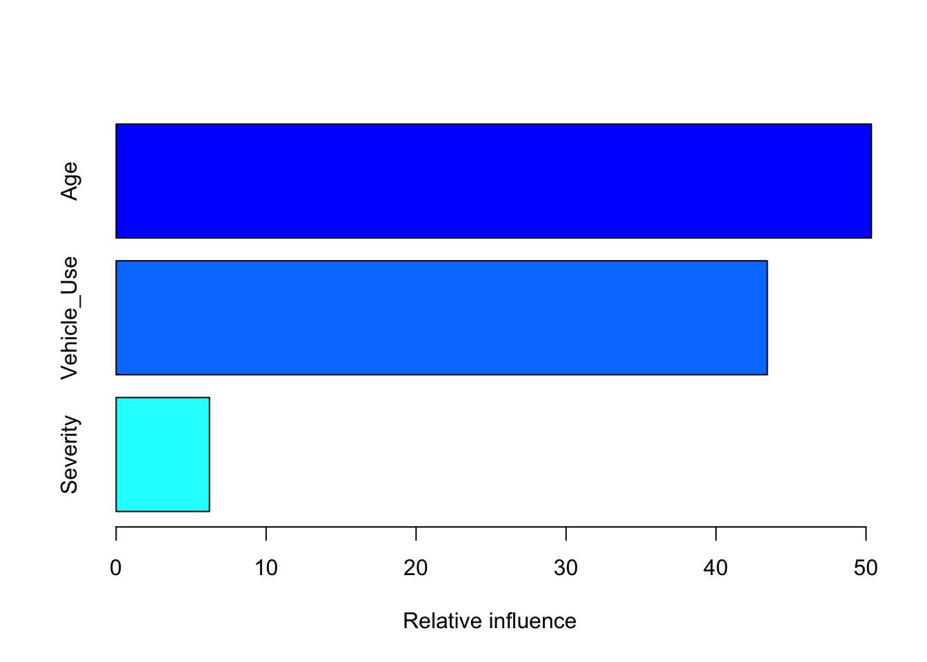

##                     var   rel.inf
## Age                 Age 50.358258
## Vehicle_Use Vehicle_Use 43.419429
## Severity       Severity  6.222313

6.4 Ensemble learning

In statistics and machine learning, ensemble methods use multiple learning algorithms to obtain better predictive performance than could be obtained from any of the constituent learning algorithms alone. Source: Wikipedia

h2o / stacking

6.5 Additional Machine Learning Techniques

xgboost: Extreme Gradient Boosting, which is an efficient implementation of gradient boosting framework. This package is its R interface. The package includes efficient linear model solver and tree learning algorithms. The package can automatically do parallel computation on a single machine which could be more than 10 times faster than existing gradient boosting packages. It supports various objective functions, including regression, classification and ranking. The package is made to be extensible, so that users are also allowed to define their own objectives easily.
TDboost: A boosted Tweedie compound Poisson model using the gradient boosting. It is capable of fitting a flexible nonlinear Tweedie compound Poisson model (or a gamma model) and capturing interactions among predictors.
glmnet: lasso, ridge, elasticnet: Extremely efficient procedures for fitting the entire lasso (least absolute shrinkage and selection operator) or elastic-net regularization path for linear regression, logistic and multinomial regression models, Poisson regression and the Cox model. Two recent additions are the multiple-response Gaussian, and the grouped multinomial. The algorithm uses cyclical coordinate descent in a path-wise fashion.
randomForest: Classification and regression based on a forest of trees using random inputs.
K-means / K-mediods: K Means Clustering is an unsupervised learning algorithm that tries to cluster data based on their similarity. Available in the base stats package